Playing with leafletR
Coming back from a bicycle ride in Tarn, I wanted to have a look at the trip. This gave me the opportunity to learn how to use the R package leafletR to obtain an HTML map using leaflet and the great projects OpenStreetMap or Thunderforest (among others).
Introduction
To use leaflet over R, two packages (at least) exist: leafletR or leaflet (developed by RStudio). After a few tests, I chose the first which directly exports a HTML/Java file that can easily been integrated in a webpage. leaflet however seems to have a nice integration for shiny.
The track was recorded through a Garmin device and I saved the six different GPX files recorded during the six different days of the ride in a directory which will be named gpx. GPX can be obtained from the web interface Garmin Connect or the web application strava (which allows you to save your tracks with a simple smartphone). I used the second one.
Installation
Installation of packages is described for (X)Ubuntu 14.04 LTS.
To obtain the desired map, I needed the following packages:
-
plotKML which was useful to read GPX files. This package depended on rgdal and sp. sp was installed using the rutteR repository as explained in this post and running the command line:
sudo apt-get install r-cran-sp
Then, rgdal (not available in the rutteR repository) needed the installation of the Ubuntu package
libgdal-dev. This was performed running the following command line in a terminal:sudo apt-get install libgdal-dev
Then, the standard R command
install.packages(c("rgdal","plotKML"))was sufficent to finish the installation of plotKML.</li>
-
leafletR was easily installed with:
install.packages("leafletR")</ul>
-
first, the GPX data are imported with plotKML. With them (and my personnal comments), I created two data frames: the first one contained the latitude and longitude of all points in the GPX files and the second one contained indications about the stop at the end of each days (latitude, longitude and elevation as indicated in the GPX files, as well as other information such as the place where we ate and slept). This is performed with the following command lines:
library(plotKML) # informations about the places where we stoped at the end of each day stopNames = c("Toulouse", "Lac de St Ferreol", "Brassac", "Murat-Sur-Vèbre", "Ambialet", "Puycelsi") stopDates = c("", "26-27/07", "27-28/07", "28-29/07", "29-30/07", "30/07-01/08") stopSleep = c("maison :)", "chez Yves et Brigitte ***","camping municipal **", "Hôtel Durand **", "La Parenthèse **", "Ancienne Auberge ****") stopEat = c("maison :)", "Le café du lac *", "Snack étape du vieux pont *", "Hôtel Durand **", "La Parenthèse **", "Le jardin des Lys ***") # collecting the list of all GPX files allGPXfiles = dir("gpx") myGPX = readGPX(paste0("gpx/",allGPXfiles[1])) # initializing the two data frames allPoints = data.frame(long=myGPX$tracks[[1]][[1]]$lon, lat=myGPX$tracks[[1]][[1]]$lat) allStops = data.frame(x=myGPX$tracks[[1]][[1]]$lat[1], y=myGPX$tracks[[1]][[1]]$lon[1], altitude=as.numeric(myGPX$tracks[[1]][[1]]$ele[1]), halte=stopNames[1], dates=stopDates[1], hébergement=stopSleep[1], restauration=stopEat[1]) # loop over GPX files to collect informations and update the data frames for (ind in setdiff(seq_along(allGPXfiles),1)) { myGPX = readGPX(paste0("gpx/",allGPXfiles[ind])) allPoints = rbind(allPoints, data.frame(long=myGPX$tracks[[1]][[1]]$lon, lat=myGPX$tracks[[1]][[1]]$lat)) allStops = rbind(allStops, data.frame(x=myGPX$tracks[[1]][[1]]$lat[1], y=myGPX$tracks[[1]][[1]]$lon[1], altitude= as.numeric(myGPX$tracks[[1]][[1]]$ele[1]), halte=stopNames[ind], dates=stopDates[ind], hébergement=stopSleep[ind], restauration=stopEat[ind])) } -
then, using the function
styleSingle, two styles are created: the first one is for the lines that will show the ride itself (red lines) and the second one is for the stops (blue dots):styTrack = styleSingle(col="darkred", lwd=3) styStops = styleSingle(col="darkblue", fill.alpha=1, rad=5)
-
finally, using these data, the map is created. With the functions
SpatialLinesandLine(s)from the R package sp and the functiontoGeoJSONa JSON file which contains information about the track is created:library(sp) tarnTour = SpatialLines(list(Lines(list(Line(allPoints)),"line1")), proj4string = CRS("+proj=longlat +ellps=WGS84")) tarnTDat1 = toGeoJSON(data=tarnTour, name="itinéraire", dest="maps/")(a file is created in the directory
maps, which is nameditinéraire.geojson). Then, another file that contains the informations about the stops is created with:tarnTDat2 = toGeoJSON(data=allStops, name="arrêts", dest="maps/")
(this file is named
maps/arrêts.geojson).And finally, the map is created using:
tarnTMap = leaflet(list(tarnTDat1, tarnTDat2), dest="maps/",
                   style=list(styTrack, styStops),
                   title="Tour du Tarn à Vélo - Juillet 2015",
                   base.map=list("osm","tls"),
                   popup=c("altitude", "halte", "dates", "hébergement",
                           "restauration"), incl.data=TRUE)
(it can be visualized opening the file
maps/Tour_du_Tarn_à_Vélo_-_Juillet_2015/Tour_du_Tarn_à_Vélo_-_Juillet_2015.html). It contains a select tool to select the map style (OpenStreetMap or Thunderforest), and a popup menu at each stop with various informations provided about the stop. The optionincl.data=TRUEallows the data to be include in the HTML file so that this file is self-content.</li> </ol>The resulting HTML page can be visualized here!
</div>
The result is dedicated to my beloved husband who organized the whole trip.
Creating the map
The map is creating using three main steps:
Processing an XL grading sheet with R
This tutorial is dedicated to
Vincent and to Erwan, the former for proposing me an interesting challenge to solve with R and the latter for his suspicious remarks about the language not being suited for this kind of task.
Disclaimer: of course, this script can not be used on a computer with Windows OS… 😉
Problem description
When correcting students’ essays, some teachers prefer filling a worksheet with detailed grading for every question in the essay (I must confess that you must be a bit mental to do it but actually… I do it). Well, this kind of detailed grading of an essay can be directly stored in a XL (yeah…) file and the teacher does not write anything on the students’ essay. The file looks like this file NotesPartiel.xls, which is provided as an example (the marks are real but the names are not). It looks like this:
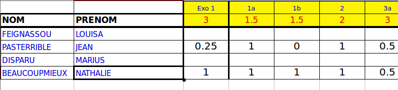
with the first row containing the questions’ numbers, the second, the questions’ full mark and then, the detailed grades for every student. The first two columns contain the students’ first and last names.
The challenge was to code an R script for creating a PDF file that contains a page with the name and detailed marks for every student. To do so, I used:
- a simple R script to manage the overall process: the script loads the XL file, loops over the rows and calls bash commands that creates separated PDF files and merges then into a single PDF file;
- a Sweave file which is used to insert expression evaluated by R and coming for the XL file into a LaTeX document.
Solution part 1: Rscript
The R script first contains a customizable part in which the user can define:
-
the file name
myfile; -
the questions’ names, which is the character vector
questions################################# Vincent : to be customized # nom du fichier myfile = "NotesPartiel.xls" # questions questions = c("exo 1", "exo 1, question a", "exo 1, question b", "exo 2", "exo 3, question a", "exo 3, question b", "exo 3, question c", "exo 4", "exo 5", "exo 3 hypothèse", "exo 3") ###############################################################################To load the data, the R package gdata is then used:
# load data
library(gdata)
notes = read.xls(myfile, sheet=1, header=TRUE)
Then, a loop is performed over the file’s rows (starting from the second one up to the last one) which:
- check that the current student has a mark (in the other case, nothing happens);
-
use the R package knitr to compile the Sweave document which creates a LaTeX (
.tex) file; -
using the function
systemrun bash commands to compile the LaTeX file with pdflatex and rename it with a name that contains the number of the current row;
library(knitr)
# run... ! first line is the total
toBeMerged = NULL
for (ind in 2:nrow(notes)) {
  if (sum(!is.na(notes[ind,3:(ncol(notes)-3)]))!=0) {
    # Sweave the document...
    knit("TraiterNotes.Rnw")
    # pdflatex
    system("pdflatex TraiterNotes.tex")
    # Move the output
    system(paste0("mv TraiterNotes.pdf TraiterNotes-",ind,".pdf"))
    if (is.null(toBeMerged)) {
      toBeMerged = paste0("TraiterNotes-",ind,".pdf")
    } else toBeMerged = paste0(toBeMerged, " TraiterNotes-", ind, ".pdf")
  }
}
Finally, all the PDF files that have been created (and those names have been merged during the processing of the previous loop into a string variable called
toBeMerged) are merged with ghostscript and all PDF files except the merged file are deleted.# Merge system(paste0("gs -dBATCH -dNOPAUSE -sDEVICE=pdfwrite -sOutputFile=finalNotes.pdf ", toBeMerged)) # Clean system(paste0("rm ", toBeMerged))Solution part 2: Sweave file
The Sweave file
TraiterNotes.Rnwis very simple. It contains a standard LaTeX header, which can be customized by the user:\documentclass{article} %%%%%%%%%%%%%%%%%%%%%%%%%%%%%%%%% Vincent : to be customized \title{Notes du devoir trucmuche} \author{Vincent X} \date{} %%%%%%%%%%%%%%%%%%%%%%%%%%%%%%%%%%%%%%%%%%%%%%%%%%%%%%%%%%%%%%%%%%%%%%%%%%%%%%% \usepackage[utf8]{inputenc} \begin{document} \pagestyle{empty}The remaining of the script contains standard R code inserted in chunks which allows the script to display a table with the detailed marks (using the R package xtable)
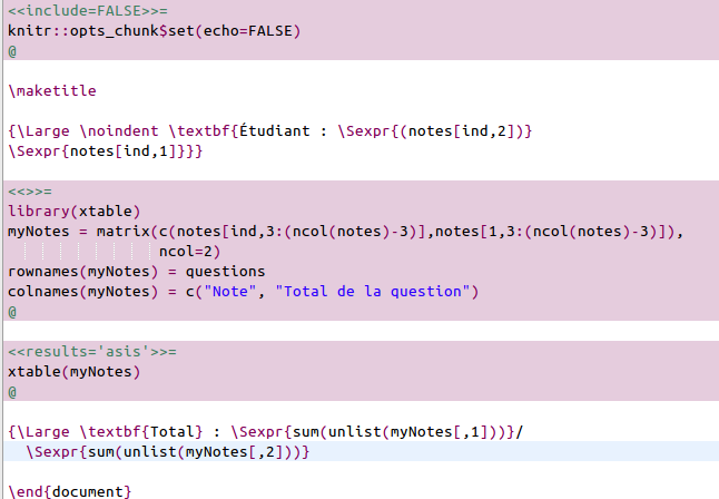 and simple texts evaluated by R thanks to the function
 Sexpr. The global knitr optionecho=FALSEis used to prevent the R script to the displayed in the PDF file.Finally, running the R script (from the directory in which the
</div>.Rmdand the.xlsfiles are saved) leads to the following PDF file finalNotes.pdf. Not very elegant programming but very handy… Vincent owes me 75 beers for that work!
Publication de SOMbrero v1.0SOMbrero v1.0 is released
 Nouveau !!! SOMbrero est désormais sur le CRAN : http://cran.r-project.org/web/packages/SOMbrero
Vous pouvez toujours tester son interface graphique en ligne : http://shiny.nathalievialaneix.eu/sombrero (SOMbrero WUI, v1.0 lié à SOMbrero v1.0) qui est aussi utilisable directement en local en installant le package.
SOMbrero est un package R destiné à réaliser l’apprentissage de cartes auto-organisatrices en version stochastique. La version 0.4-1 du package contenant l’implémentation pour données numériques (avec graphiques, fonctions de qualité et super-classification), pour les tables de contingence (“korresp”) et pour les données décrites par des dissimilarités (“relational”) est décrite sur cette page (voir la page en anglais).
Présentation de SOMbrero aux 2èmes rencontres R à Lyon (28 juin 2013) :
<strong>SOMbrero</strong> is now on CRAN: http://cran.r-project.org/web/packages/SOMbrero
You can visit its Web User Interface: http://shiny.nathalievialaneix.eu/sombrero (SOMbrero WUI, v1.0 related to SOMbrero v1.0). The web user interface can also be used directly from the package with the function sombreroGUI().
<strong>SOMbrero</strong> is an R package dedicated to online (also called “on-line”) Self-Organizing Maps. The version 0.4-1 of the package can be used to train SOMs for numeric datasets, contingency tables (algorithm “KORRESP” which is illustrated on the “presidentielles 2002” dataset: see user-friendly documentation) or for dissimilarity data (relational SOM, illustrated on a graph from the novel Les Misérables). It contains many graphical functions for helping the user to interpret the results, as well as quality functions and super-clustering.
Maintainer: Nathalie Villa-Vialaneix (SAMM, Université Paris 1)
Authors: Laura Bendhaïba, Madalina Olteanu, Nathalie Villa-Vialaneix
The authors are grateful to Nicolas for his help with the implementation of the “korresp” algorithm, to Patrick for the original implementation of the “korresp” algorithm on SAS and to Marie for useful discussions.
Important warning: This package has been implemented only by girls. Default colors may not be suited for men.
The package has been presented at 2èmes rencontres R (Lyon, France, on June 28th, 2013). The article (abstract, in French) can be downloaded here. You can also have a look at the slides (in French):
Analyse du profil des étudiants d’un MOOC
Cette analyse a été réalisée en collaboration avec Avner.
Cette page présente une analyse statistique effectuée sur le profil des étudiants du MOOC « Fondamentaux en Statistique » qui a été publié sur la plate-forme France Université Numérique (FUN) le 16 janvier 2014 pour une durée de 5 semaines. Un questionnaire auto-déclaratif conçu par FUN et proposé aux étudiants lors de leur inscription a permis d’obtenir des informations sur les étudiants. Nous présentons ici une analyse simple de leur profil. Cette analyse est réalisée avec le logiciel statistique libre R et les packages :
library(OpenStreetMap)
library(ggplot2)
library(xtable)
library(FactoMineR)
L’analyse requiert l’importation dans l’espace de travail de R des fichiers anonymousStudents-FUN.csv (fichier contenant les informations sur les étudiants obtenues à partir du questionnaire auto-déclaratif) et addresses-FUN.csv (fichier contenant les informations sur les étudiants obtenues à partir des déclarations et des API de géo-localisation de Google Map et de Open Street Map). Les fichiers sont importés à partir des commandes :
students = read.csv("anonymousStudents-FUN.csv", stringsAsFactor=FALSE,
                     fileEncoding="UTF8")
addresses = read.csv("addresses-FUN.csv", fileEncoding="UTF8")
Le nombre de répondants au questionnaire est 6918.
Analyse du sexe
Dans cette partie, nous étudions tout d’abord le sexe des étudiants dont la répartition est donnée dans le tableau ci-dessous :
students$gender[students$gender%in%c("","None")] = NA
outGender = as.matrix(table(students$gender))
rownames(outGender) = c("Femmes", "Hommes")
colnames(outGender) = "Effectifs"
print(xtable(outGender), type="html")
| Effectifs | |
|---|---|
| Femmes | 2108 |
| Hommes | 4493 |
outGender = outGender/sum(!is.na(students$gender))*100
colnames(outGender) = "Fréquences (%)"
print(xtable(outGender, digits=1), type="html")
| Fréquences (%) | |
|---|---|
| Femmes | 31.9 |
| Hommes | 68.1 |
Ceci nous montre que moins de $\frac{1}{3}$ des étudiants sont des étudiantes.
Analyse de l’âge
Cette partie s’intéresse à l’âge des étudiants :
students$age = 2013 - as.numeric(students$year_of_birth)
Le nombre d’étudiants ayant déclaré avoir moins de 13 ans est 38 et le nombre d’étudiants ayant déclaré avoir plus de 100 ans est 2. Ces étudiants sont supprimés de l’analyse :
students$age[students$age<=13|students$age>100] = NA
ageSummary = as.matrix(summary(students$age))
colnames(ageSummary) = "valeur"
rownames(ageSummary) = c("minimum", "Q1", "médiane", "moyenne", "Q3",
                          "maximum", "valeur manquante")
print(xtable(ageSummary, digits=2), type="html")
| valeur | |
|---|---|
| minimum | 14.00 |
| Q1 | 26.00 |
| médiane | 34.00 |
| moyenne | 35.57 |
| Q3 | 43.00 |
| maximum | 84.00 |
| valeur manquante | 439.00 |
Le nombre d’étudiants pour lequel l’âge est connu est donc 6479, ce qui correspond à 93.65% des étudiants ayant rempli le questionnaire. La figure ci-dessous montre la répartition de l’âge des étudiants :
p = ggplot(students, aes(x=age)) +
  geom_histogram(aes(y=..density..), binwidth=1) +
  geom_density(linewidth=2, colour="darkred") + xlab("Âge") + ylab("") +
  theme(panel.background=element_rect(fill="white", colour="grey"))
print(p)
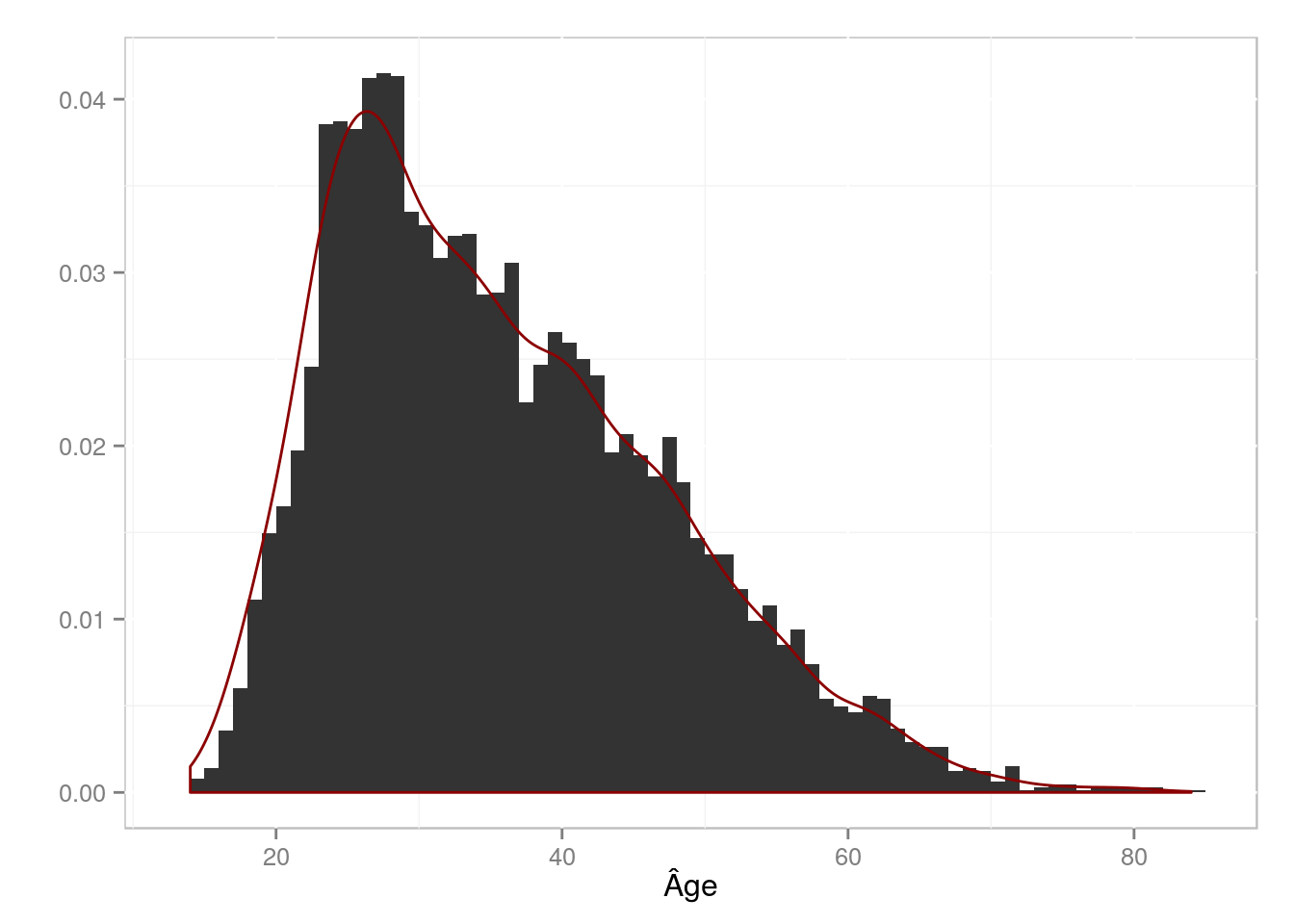
Celle-ci permet de constater que beaucoup d’étudiants ont entre 25 et 35 ans, avec des étudiants beaucoup plus âgés (l’âge maximum étant 84 ans).
Analyse du niveau d’études
La répartition des divers niveaux d’études parmi la population des étudiants est donnée dans le tableau ci-dessous :
students$level_of_education[students$level_of_education=="a"] =
  "Licence professionnelle"
students$level_of_education[students$level_of_education=="b"] = "Licence"
students$level_of_education[students$level_of_education=="el"] = "Brevet"
students$level_of_education[students$level_of_education=="hs"] = "Baccalauréat"
students$level_of_education[students$level_of_education=="jhs"] = "DUT/BTS"
students$level_of_education[students$level_of_education=="m"] = "Master"
students$level_of_education[students$level_of_education=="none"] =
  "Aucun"
students$level_of_education[students$level_of_education=="other"] = "Autre"
students$level_of_education[students$level_of_education=="p"] = "Doctorat"
students$level_of_education[students$level_of_education%in%c("","None")] = NA

students$level_of_education = factor(students$level_of_education,
       levels=c("Aucun", "Brevet", "Baccalauréat", "DUT/BTS",
                "Licence professionnelle", "Licence", "Master", "Doctorat",
                "Autre"),
       ordered=TRUE)
outEducation = as.matrix(table(students$level_of_education))
colnames(outEducation) = "Effectif"
print(xtable(outEducation), type="html")
| Effectif | |
|---|---|
| Aucun | 27 |
| Brevet | 65 |
| Baccalauréat | 497 |
| DUT/BTS | 546 |
| Licence professionnelle | 178 |
| Licence | 967 |
| Master | 3208 |
| Doctorat | 937 |
| Autre | 188 |
Le nombre d’étudiants pour lequel on connaît le niveau d’études est donc 6613 soit environ 95.59% des étudiants ayant rempli le questionnaire. Parmi ceux-ci, la fréquence d’étudiants de master est 48.51%. Les personnes suivant le cours le suivent donc probablement dans le cadre d’un enrichissement personnel de leur niveau de formation puisque le type d’enseignement dispensé dans le cours « Fondamentaux en Statistique » se situe généralement en premier cycle d’un cursus universitaire en France.
Relation entre âge et niveau d’études
Une analyse factorielle des correspondances (AFC) permet de préciser la relation entre âge et niveau d’études (voir « Saporta (1990) Probabilités, analyse des données et statistique. Editions Technip » pour une introduction à l’AFC) :
breakDates = c(1900,1961,1967,1972,1976,1980,1983,1986,1988,1991,2013)
students$age_class = cut(students$age, breaks=2013-breakDates,
                          labels=c("22 ans et moins", "23-25 ans",
                                   "26-27 ans", "28-30 ans", "31-33 ans",
                                   "34-37 ans", "38-41 ans", "42-46 ans",
                                   "47-52 ans", "53 ans et plus"))
curDF = na.omit(data.frame(age=students$age_class,
                            education=students$level_of_education))
resCA = CA(table(curDF), graph=FALSE)
plot(resCA, axes=1:2, title="")
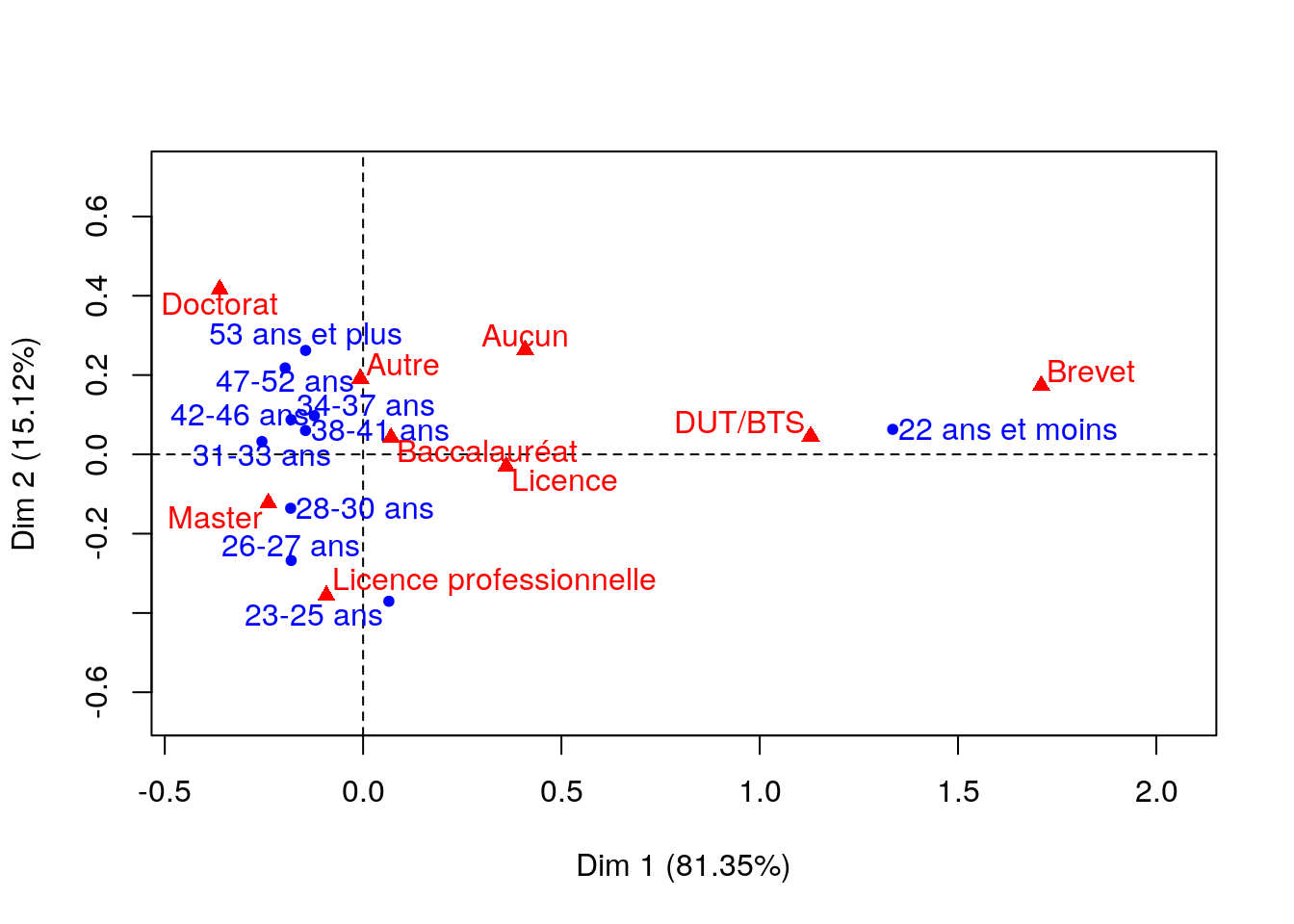
81.35% de la variance est expliquée par l’axe 1 et 15.12% par l’axe 2. Le premier plan factoriel représente donc 96.47% de la variance : de manière claire, celui-ci sépare les plus jeunes (moins de 22 ans, qui sont probablement encore dans le système scolaire) du reste des autres étudiants. Ils ont la particularité d’avoir un plus faible niveau d’études (qui s’explique au moins en partie par leur âge), Brevet et DUT/BTS en particulier. Le deuxième axe oppose les étudiants ayant suivi des études plutôt courtes et professionnalisantes (licence professionnelle) qui sont plutôt jeunes (moins de 30 ans) aux les étudiants ayant suivi des études plus longues (doctorat) et qui sont plus âgés (plus de 47 ans).
Analyse de la localisation géographique
Étudiants français
Dans un premier temps, nous analysons la localisation géographique des étudiants habitant en France :
coordFrance = addresses[which(addresses$country=="France"),]
Le nombre d’étudiants ayant déclaré être localisé en France est 2826. Les principales villes où sont localisés les étudiants sont listées ci-dessous :
frenchTable = table(coordFrance[,3])
outFrench = as.matrix(head(frenchTable[order(frenchTable,decreasing=TRUE)],
                            n=11))
colnames(outFrench) = "Effectif"
outFrench = xtable(outFrench, align="|l|c|")
print(outFrench, type="html")
| Effectif | |
|---|---|
| Paris | 388 |
| Lyon | 49 |
| Marseille | 46 |
| Toulouse | 41 |
| Montpellier | 33 |
| Strasbourg | 31 |
| Bordeaux | 26 |
| Nantes | 23 |
| Versailles | 21 |
| Nice | 20 |
| Rennes | 20 |
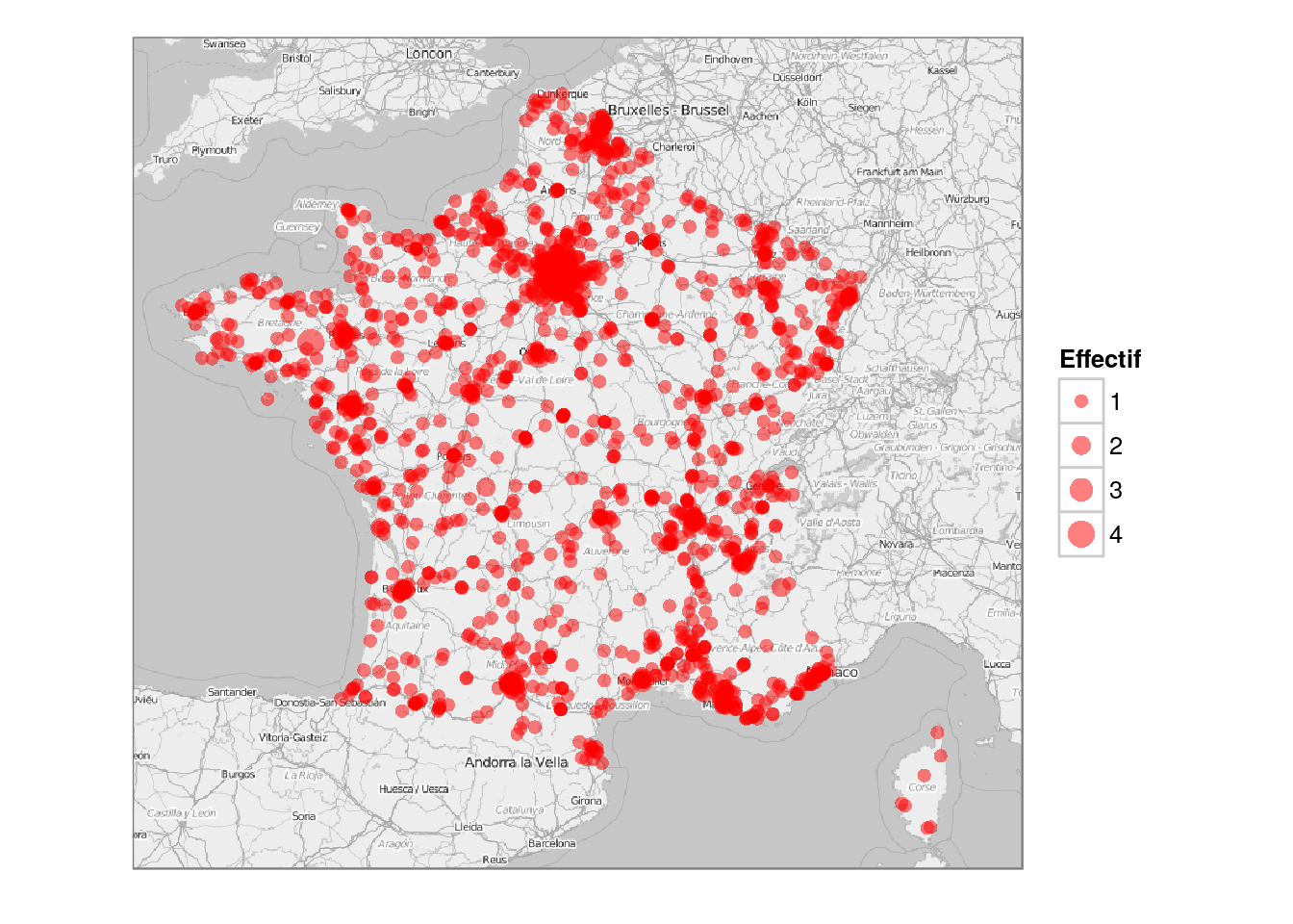
De manière plus précise, la localisation géogrpahique des étudiants français peut être visualisée sur une carte obtenue à partir des fonds de carte de Open Street Map (l’aire des disques est proportionnelle à l’effectif) :
franceData = data.frame(coordFrance,
                         students[which(addresses$country=="France"),])
onlyUniqueCoord = unique(coordFrance)
onlyUniqueCoord = onlyUniqueCoord[which(!is.na(onlyUniqueCoord[,1])),]
# remove strange point
onlyUniqueCoord = onlyUniqueCoord[-c(2596),]
mapDF = data.frame(projectMercator(onlyUniqueCoord[,1],
                                    onlyUniqueCoord[,2]))
mapDF$size = sapply(1:nrow(onlyUniqueCoord), function(ind)
  sum(coordFrance[,1]==onlyUniqueCoord[ind,1] &
        coordFrance[,2]==onlyUniqueCoord[ind,2], na.rm=TRUE))
frenchMap = openmap(c(51.700,-5.669), c(41,11), type="osm-bw")
p = autoplot(frenchMap) +
  geom_point(aes(x=x,y=y,size=size), colour=heat.colors(20,alpha=0.5)[1],
             data=mapDF) +
  theme_bw() + scale_size_area(max_size=5) + labs(size="Effectif") +
  theme(axis.title.x=element_blank(), axis.ticks=element_blank(),
        axis.text.x=element_blank(), axis.title.y=element_blank(),
        axis.text.y=element_blank())
print(p)
Ensemble des étudiants
On analyse maintenant la localisation géographique des étudiants du monde entier.
worldData = data.frame(addresses[!is.na(addresses[,1]),],
                        students[!is.na(addresses[,1]),])
Le nombre d’étudiants dont on connait la localisation géographique est 3730 ce qui correspond à environ 53.92% des étudiants ayant répondu au questionnaire. Par ailleurs, le nombre d’étudiants localisés en Franche correspond à environ 75.76% des étudiants dont on connaît la localisation.
Les principaux pays dont sont issus les étudiants sont :
worldTable = table(worldData$country)
outWorld = as.matrix(head(worldTable[order(worldTable,decreasing=TRUE)], n=14))
colnames(outWorld) = "Effectif"
outWorld = xtable(outWorld, align="|l|c|")
print(outWorld, type="html")
| Effectif | |
|---|---|
| France | 2826 |
| Morocco | 94 |
| United States | 78 |
| Algeria | 60 |
| Belgium | 45 |
| Senegal | 39 |
| Canada | 38 |
| Cameroon | 36 |
| Tunisia | 33 |
| Switzerland | 29 |
| Côte d’Ivoire | 28 |
| Mali | 21 |
| Benin | 20 |
| Burkina Faso | 20 |
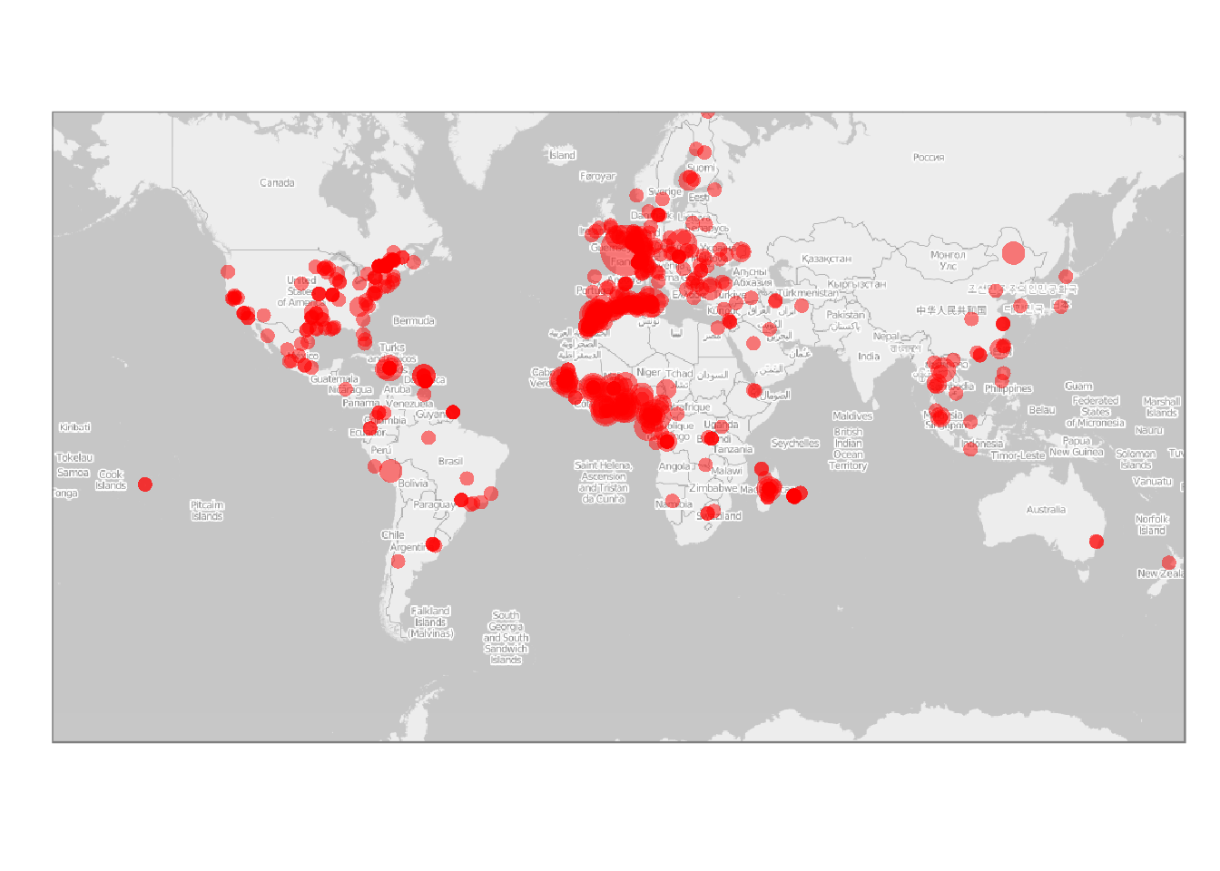
ce qui permet d’identifier qu’un grand nombre d’étudiants localisés à l’étranger sont issus de l’Afrique francophone. De manière plus complète, la localisation géographique des étudiants est donnée par la carte suivante (l’aire des disques est proportionnelle au $\log_2$ de l’effectif afin de ne pas sur-représenter la France métropolitaine qui est représentée par un seul point) :
indParis = which(worldData[,3]=="Paris")[1]
worldData[which(worldData[,4]=="France"),1:2] =
  worldData[indParis,1:2]
onlyUniqueCoord = unique(worldData[,1:2])
mapDF = data.frame(projectMercator(onlyUniqueCoord[,1],
                                    onlyUniqueCoord[,2]))
mapDF$size = sapply(1:nrow(onlyUniqueCoord), function(ind)
  log2(sum(worldData[,1]==onlyUniqueCoord[ind,1] &
        worldData[,2]==onlyUniqueCoord[ind,2]))+1)

worldMap = openmap(c(70,-179), c(-70,179), type="osm-bw")

p = autoplot(worldMap) +
  geom_point(aes(x=x,y=y,size=size), colour=heat.colors(20,alpha=0.5)[1],
             data=mapDF) + theme_bw() + scale_size_area(max_size=10) +
  theme(axis.title.x=element_blank(), axis.ticks=element_blank(),
        axis.text.x=element_blank(), axis.title.y=element_blank(),
        axis.text.y=element_blank(), legend.position="none")
print(p)
Installer RStudio Serveur sur Ubuntu ServeurInstalling RStudio Server on Ubuntu Server
This tutorial describes the different steps required to install RStudio Server on Ubuntu Server (version 14.04 LTS). It is widely inspired from the official installation instructions
Installing R
First, R must be installed on the server. The best way to do so is to proceed as described on this page, that is:
-
edit the file
/etc/apt/sources.listto add your favorite CRAN repositorydeb http://cran.univ-paris1.fr/bin/linux/ubuntu trusty/
(cran.univ-paris1.fr is my favorite CRAN repository because it is managed by my fabulous former lab)</li>
-
add the corresponding GPG keys to your list of keys:
gpg --keyserver keyserver.ubuntu.com --recv-key E084DAB9
gpg -a --export E084DAB9 | sudo apt-key add -
-
reload the package list and install R
sudo apt-get update
sudo apt-get install r-base r-base-dev
</ul>
The best way to install packages is to use the up-to-date packages from RutteR PPA. Install the PPA using:
sudo add-apt-repository ppa:marutter/rrutter
sudo apt-get update
and packages can simply be installed using
sudo apt-get install r-cran-reshape2
for instance (for installing the excellent package reshape2. It is better to install the packages as an admin because they will be available for all users and not only the current user.
Installing RStudio Server
The free version of RStudio Server can be found at this link. The installation is performed by first installing two additional packages (the first one to ease the installation of deb packages and the second one to manage security options in RStudio Server:
sudo apt-get install gdebi-core libapparmor1
Then, the package is downloaded and installed using:
wget http://download2.rstudio.org/rstudio-server-0.98.1091-amd64.deb
sudo gdebi rstudio-server-0.98.1091-amd64.deb
At this step, RStudio Server is maybe accessible at http://my-domain.org:8787. If not (and/or if you want to create a virtual host to access RStudio Server more easily), read the next section.
Last details to check
If you are using a firewall on your server, make sure that the port 8787 is open. In my case, it is managed with shorewall (see this post, in French) and the port can be open by editing the file /etc/shorewall/rules and adding the following line
ACCEPT net $FW tcp 8787
before reloading the firewall configuration
sudo service shorewall restart
A virtual host can be set for accessing RStudio Server at an URL of the type http://rstudio.my-domain.org by
-
creating a
Afield in OVH manager to redirect the URLhttp://rstudio.my-domain.orgto my server’s IP -
adding the entry
http://rstudio.my-domain.orgin the file/etc/hosts -
creating a virtual host with the port redirection. For this step, the following modules must be enabled in apache:
sudo a2enmod proxy proxy_connect proxy_http
sudo service apache2 reload
and a file
/etc/apache2/site-available/rstudio.confwithServerAdmin me@my-domain.org ServerName rstudio.my-domain.org ProxyPass / http://127.0.0.1:8787/ ProxyPassReverse / http://127.0.0.1:8787/
must be created. It is activated with:
sudo a2ensite rstudio
sudo service apache2 reload
It seems that SSL access to RStudio Server is not available for the free version.
Users allowed to use RStudio Server are those with a UID larger than 100. Any user created with the command linesudo adduser trucmuche
are allowed to connect to a RStudio Server session with their username (
trucmuche) and the password given at the account creation.</li> </ul>
</div>

