Inspired by this post, I wanted to use Google Scholar data to put nice images on my professional website (girly habit). This post explains how I combined the functions available in the R package scholar with additional analyses (partially inspired from the script available at this link, which in my case results in a cannot open the connection error message) to generate a few informative graphics.

Get a summary of all publications

Using the function get_publications in the package scholar, you can obtain a summary (title, authors, journal, volume and issue numbers, number of citations, year and google scholar ID) of all the paper a given author has published. However, the default publication displayed on the first page of an author’s google scholar profile is 20 so the function only returns the first 20 citations. A solution could have been to modify the package’s function to add a &pagesize=1000 (supposing that the author has less than 1000 publications, which seems reasonable enough) in the parsed URL. I chose a slightly different method, directly using the package function and that relies on the use of the argument cstart which tells from which citation the data acquisition should start. Hence, looping over this argument, we can retrieve all publications, 20 at each call of the function:

get_all_publications = function(authorid) {
  # initializing the publication list
  all_publications = NULL
  # initializing a counter for the citations
  cstart = 0
  # initializing a boolean that check if the loop should continue
  notstop = TRUE
  
  while (notstop) {
    new_publications = try(get_publications(my_id, cstart=cstart), silent=TRUE)
    if (class(new_publications)=="try-error") {
      notstop = FALSE
    } else {
      # append publication list
      all_publications = rbind(all_publications, new_publications)
      cstart=cstart+20
    }
  }
  return(all_publications)
}

In my case, the use of this function gives:

library(scholar)
my_id = "MY GOOGLE SCHOLAR ID"
all_publications = get_all_publications(my_id)
dim(all_publications)
# [1] 122   8
table(all_publications$year)
# 2004 2005 2006 2007 2008 2009 2010 2011 2012 2013 2014 2015 
#    1    4    7    7    8    9    7    9   12   11   18    7 
summary(all_publications$cites)
#    Min. 1st Qu.  Median    Mean 3rd Qu.    Max. 
#   0.000   0.000   0.000   5.566   5.000 140.000

Find all co-authors

From the previously obtained publication list, we can also retrieve all co-authors. This is done by using the column author and by splitting it on the character “, “. Additionally, for long authorship lists, the author "..." has also to be removed (which biases a bit the list actually…):

get_all_coauthors = function(my_id, me=NULL) {
  all_publications = get_all_publications(my_id)
  if (is.null(me))
    me = strsplit(get_profile(my_id)$name, " ")[[1]][2]
  # make the author list a character vector
  all_authors = sapply(all_publications$author, as.character)
  # split it over ", "
  all_authors = unlist(sapply(all_authors, strsplit, ", "))
  names(all_authors) = NULL
  # remove "..." and yourself
  all_authors = all_authors[!(all_authors %in% c("..."))]
  all_authors = all_authors[-grep(me, all_authors)]
  # make a data frame with authors by decreasing number of appearance
  all_authors = data.frame(name=factor(all_authors, 
    levels=names(sort(table(all_authors),decreasing=TRUE))))
}

The argument me is used to remove yourself from your own co-authorship list. By default, it will use your family name as recorded in your google scholar profile (if your family name is the second word of your whole name). In my case, I used two names in my publications so manually provided the argument:

all_authors = get_all_coauthors(my_id, me="PART OF MY NAME")

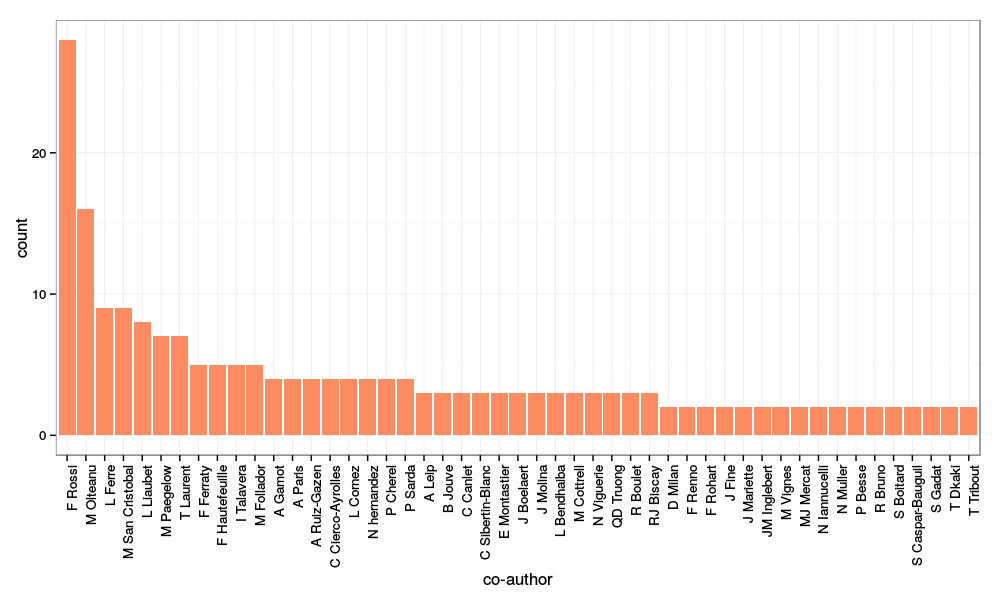
After a bit of cleaning up (removing co-authors who are only cited once, fixing some encoding issues…), I obtained the following image:

with (among other commands for cleaning up the data a bit):

main_authors = all_authors[all_authors$name %in% names(which(table(all_authors$name)>1)), ]
library(ggplot2)
p = ggplot(main_authors, aes(x=name)) + geom_bar(fill=brewer.pal(3, "Set2")[2]) +
  xlab("co-author") + theme_bw() + theme(axis.text.x = element_text(angle=90, hjust=1))
print(p)

Analysis of the words in the abstracts

Finally, looping over the publication IDs, we can retrieve all the abstracts of the publication list to make a basic text mining analysis. To do so, I used the package XML which provides many functions for web scraping. I first defined a function to get one article’s abstract from its google ID (and the author’s google ID):

get_abstract = function(pub_id, my_id) {
  print(pub_id)
  paper_url = paste0("http://scholar.google.com/citations?view_op=view_citation&hl=fr&user=",
                     my_id, "&citation_for_view=", my_id,":", pub_id)
  paper_page = htmlTreeParse(paper_url, useInternalNodes=TRUE, encoding="utf-8")
  paper_abstract = xpathSApply(paper_page, "//div[@id='gsc_descr']", xmlValue)
  return(paper_abstract)
}

Then, looping over the data frame all_publications that have been previously retrieved from google scholar, we obtain the list of all abstracts.

get_all_abstracts = function(my_id) {
  all_publications = get_all_publications(my_id)
  all_abstracts = sapply(all_publications$pubid, get_abstract, my_id=my_id)
  return(all_abstracts)
}

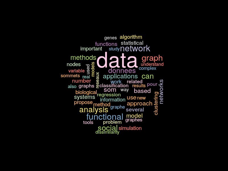
Then, the package tm is used to obtain a publication/term matrix and finally a term frequency matrix that can be processed with the package wordcloud to obtain

library(XML)
all_abstracts = get_all_abstracts(my_id)
library(tm)
# transform the abstracts into "plan text documents"
all_abstracts = lapply(all_abstracts, PlainTextDocument)
# find term frequencies within each abstract
terms_freq = lapply(all_abstracts, termFreq, 
                    control=list(removePunctuation=TRUE, stopwords=TRUE, removeNumbers=TRUE))
# finally obtain the abstract/term frequency matrix
all_words = unique(unlist(lapply(terms_freq, names)))
matrix_terms_freq = lapply(terms_freq, function(astring) {
  res = rep(0, length(all_words))
  res[match(names(astring), all_words)] = astring
  return(res)
})
matrix_terms_freq = Reduce("rbind", matrix_terms_freq)
colnames(matrix_terms_freq) = all_words
# deduce the term frequencies
words_freq = apply(matrix_terms_freq, 2, sum)
# keep only the most frequent and after a bit of cleaning up (not shown) make the word cloud
important = words_freq[words_freq > 10]
library(wordcloud)
wordcloud(names(important), important, random.color=TRUE, random.order=TRUE,
          color=brewer.pal(12, "Set3"), min.freq=1, max.words=length(important), scale=c(3, 0.3))