This tutorial is dedicated to Tibo who showed me how to use OpenStreetMap with R in the first place and gratefully sent me his script. The tutorial will explain first how to install the package OpenStreetMap under linux (which is actually a bit tricky) and will then explain how to use it to draw a map with the open online map OpenStreetMap through R.

Installing the package OpenStreetMap in R

I am using R version 3.0.1 (2013-05-16) — “Good Sport” on Ubuntu 12.04. The R version is thus not that of the ubuntu repository. To install the package OpenStreetMap, I proceeded as follows:

• first, I installed a few additional ubuntu packages:

  sudo apt-get install libproj-dev libgdal1-dev

• then, I installed open jdk version 7:

  sudo apt-get remove --purge openjdk-6-*
  sudo apt-get autoremove
  audo apt-get install openjdk-7-*

  and updated R java configuration:

  sudo R CMD javareconf

• finally, I was able to install the R package OpenStreetMap from R

  install.packages("OpenStreetMap")

  (which requires the packages rJava and rgdal that had caused errors before I did the previously described configurations).</li> </ul>

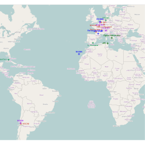
  Using OpenStreetMap

  As an example, I tried to produce a map where the last conferences I gave are located. To do so:

  • the first step is to download the map from OpenStreetMap (or another open map server). This is done by first finding the coordinates of the upper left corner and of the lower right corner on the map (on OpenStreetMap, you can use the “export” menu):

    conf.map = openmap(c(60,-90),c(-45,45),type="osm")

  • the second step is to find the coordinates of the conference places. I give the example below for the year 2013 (Toulouse, Tenerife, Bruges, Lyon). To do so, you can once again use the “export” menu and then the following command lines in R

    coord.conferences = rbind(c(-16.5,28.4),c(3.2,51.2),c(-70.6,-33.4),c(4.8,45.7))

  • then, the coordinates have to be properly converted into spatial points with proper Coordinate Reference System:

    proj4string(coord.conferences) = CRS("+proj=longlat +ellps=WGS84")
    sp.conferences = spTransform(coord.conferences,CRS("+proj=merc +a=6378137
      +b=6378137 +lat_ts=0.0+lon_0=0.0 +x_0=0.0 +y_0=0 +k=1.0 +units=m
      +nadgrids=@null +no_defs"))

  • then the map and the points are plotted:

    plot(conf.map,raster=TRUE)
    sapply(1:nrow(sp.conferences), function(ind) plot(xyb[ind,],add=TRUE,col="blue",
                                                      lwd=2,pch=19))

  • and finally, the labels of the points are added:

    sp.conferences.coord = coordinates(sp.conferences)
    conferences.names = c("IWANN","JdS, EGC","ESANN","Rencontres R")
    sapply(1:nrow(sp.conferences.coord), function(ind)
      text(sp.conferences.coord[ind,1],sp.conferences.coord[ind,2],
      conferences.names[ind],adj=1,pos=3,lwd=2,cex=0.7,col="blue"))

  After having added a few more conferences/seminars, I finally obtained the following map:

  Another example

  The map of the main places for the Journées de Statistique de Toulouse:

  

  has been made with the following command lines:

  ## Made by Thibault Laurent (for http://jd2013.sfds.asso.fr)
  # http://www.tse-fr.eu/index.php?option=com_wrapper&Itemid=398
  
  require("OpenStreetMap")
  
  ## Select the bounding box of the map from the upper left corner to the lower
  # right corner
  ## Then select the type of map, from one of those:
  
  type.map=c("osm", "osm-bw", "maptoolkit-topo", "waze", "mapquest",
  "mapquest-aerial", "bing", "stamen-toner", "stamen-terrain",
  "stamen-watercolor", "osm-german", "osm-wanderreitkarte", "mapbox", "esri",
  "esri-topo", "nps", "apple-iphoto", "skobbler", "cloudmade-", "hillshade",
  "opencyclemap", "osm-transport", "osm-public-transport", "osm-bbike",
  "osm-bbike-german")
  
  map=openmap(c(43.611522,1.428533), c(43.598903,1.461059),type=type.map[1])
  
  ## Locate the main places of the conference
  xy.1=c(1.431892,43.609747)
  xy.2=c(1.443877,43.604436)
  xy.3=c(1.455493,43.610231)
  xy.4=c(1.442447,43.600927)
  xy.5=c(1.440507,43.610111)
  xy.6=c(1.444758,43.604443)
  xy.7=c(1.449647,43.606678)
  # Create a spatial object and define the coordinate reference system
  xy=rbind(xy.1,xy.2,xy.3,xy.4,xy.5,xy.6,xy.7)
  xya=SpatialPoints(xy)
  proj4string(xya)=CRS("+proj=longlat +ellps=WGS84")
  xyb=spTransform(xya,CRS("+proj=merc +a=6378137 +b=6378137 +lat_ts=0.0
  +lon_0=0.0 +x_0=0.0 +y_0=0 +k=1.0 +units=m +nadgrids=@null +no_defs"))
  
  ## Plot the map and the points
  plot(map,raster=TRUE)
  plot(xyb[1,],add=TRUE,col="darkred",lwd=4)
  plot(xyb[2:7],add=TRUE,col="darkred",lwd=2)
  
  ## Add text
  xy=coordinates(xyb)
  names.xy=c("ESC Toulouse \n (lieu de la conférence)",
  "Mairie de Toulouse \n Salle des illustres, \n entrée par la cour Henri IV
  (réception le lundi)",
  "Médiathèque José-Cabanis \n Espaces Vanel \n (repas de gala le mercredi)",
  "Librairie Mona Lisait \n Rencontre avec Guy Limone \n (jeudi 30 mai)",
  "Café chez ta mère \n Rencontre des jeunes statisticiens
  (café de la statistique le jeudi)",
  "Donjon du Capitole \n Départ de la visite de Toulouse \n(mercredi 28 mai)",
  "Place d'Arménie \n(retour des visites \n du mercredi)")
  text(xy[1,1],xy[1,2],names.xy[1],adj=1,pos=3,lwd=1.5)
  text(xy[2,1],xy[2,2],names.xy[2],adj=1,pos=2,lwd=1.5)
  text(xy[3,1],xy[3,2],names.xy[3],adj=1,pos=1,lwd=1.5)
  text(xy[4:5,1],xy[4:5,2],names.xy[4:5],adj=1,pos=1,lwd=1.5)
  text(xy[6,1]+160,xy[6,2],names.xy[6],adj=1,pos=3,lwd=1.5)
  text(xy[7,1],xy[7,2],names.xy[7],adj=1,pos=3,lwd=1.5)

  </div>